Fiveable
Fiveable
crams
AP Statistics
Find gaps with guided practice
Guided practice grid visualization
Table of Contents

📊ap statistics review

5.3 The Central Limit Theorem

Verified for the 2025 AP Statistics examCitation:

Definition

The Central Limit Theorem is often tested on free response questions dealing with quantitative data (means). Now, you cannot assume that the sample is normally distributed. The question must either explicitly state so, or you have to follow the central limit theorem.

The Central Limit Theorem states that if a sample size (n) is large enough, the sampling distribution of the sample mean will be approximately normal, regardless of the shape of the population distribution. In general, a sample size of n > 30 is considered to be large enough for the Central Limit Theorem to hold. 🔔

It's also important to note that for the Central Limit Theorem to apply, the samples must be independent of each other and the sample must be a simple random sample. Additionally, it is generally recommended to use the Central Limit Theorem only for continuous variables, as it may not hold for discrete variables with small sample sizes.

To summarize, for a quantitative sample to be normally distributed according to the Central Limit Theorem, it should meet the following criteria:

  • The sample size (n) is large enough (usually n > 30).
  • The samples are independent of each other.
  • The sample is a simple random sample.

Example

Use the Central Limit Theorem when calculating the probability about a mean or average.

For example, if a question asks for the probability about the mean size of fish, you cannot assume that the sample of fish, say in a pond, is greater than 30 unless the problem states so.

In this question, reasoning might include that since the sample of fish is 40, which is greater than 30, it is approximately normal. This is because according to the central limit theorem, if n is large, then the sample is approximately normally distributed. Additionally, you must state that the samples are independent of each other.  This is true for both quantitative and categorical data (and the statement is the same). 

You must explicitly state that you assumed the sample is normally distributed because of the central limit theorem.

The picture below shows what happens as you increase your sample size. The smallest triangle is a sample size of 5 and the tallest is a sample size of 100. 🔺
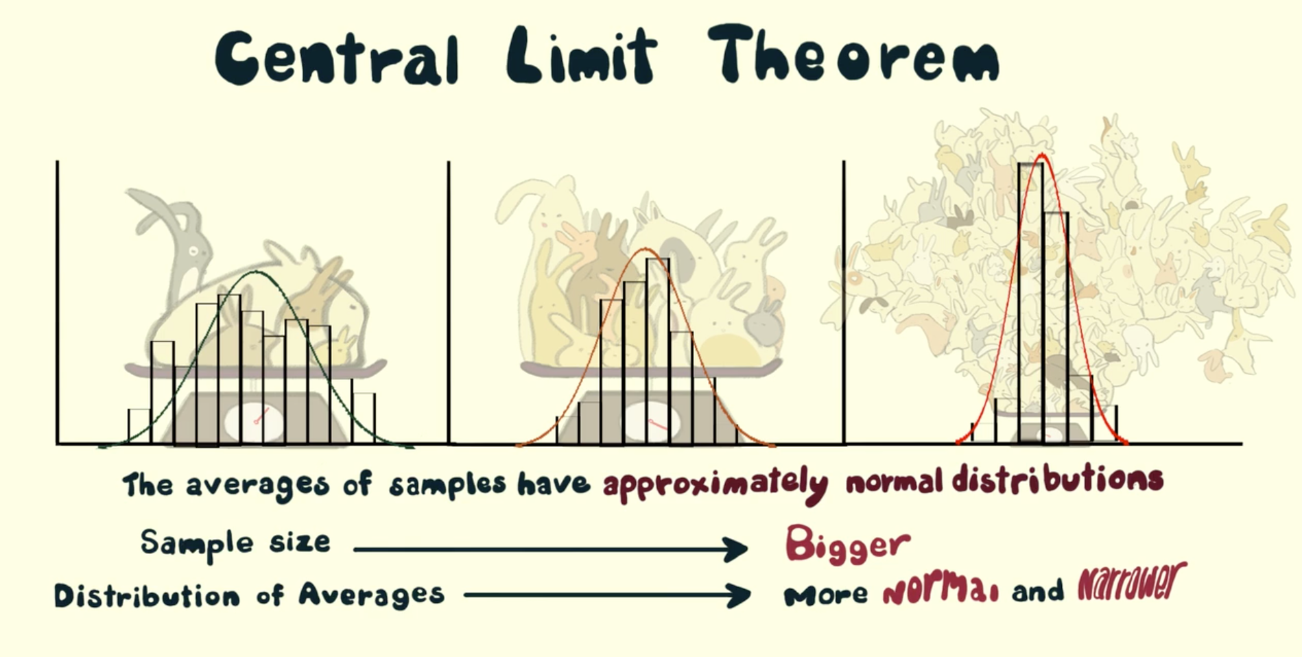
Source: SurgeForce Demo

Bigger is Better!

With sampling distributions, the larger the sample size, the less spread the curve is going to have. This is because the larger a sample is, the more the sampling distribution is going to hone in on the true population parameter

Think of this... if you flip a coin 6 times, the proportion of heads you get is likely to be greater than or less than 0.5 (the data is somewhat skewed). However, once you flip the coin 50, 100, 1000 times, it is very unlikely that the proportion of heads is going to be much different from the true population proportion, which we know is 0.5.  

Due to this concept, the larger the sample size, the better.  A large sample size allows us to hone in on the population parameter (either 𝝁 or 𝝆), which is EXACTLY what we are after when using a sampling distribution. 😄

Key Terms to Review (9)

Central Limit Theorem: The Central Limit Theorem (CLT) states that the sampling distribution of the sample mean approaches a normal distribution as the sample size increases, regardless of the population's distribution, given that the samples are independent and identically distributed. This theorem is crucial because it enables statisticians to make inferences about population parameters even when the population distribution is not normal, thereby connecting to hypothesis testing, confidence intervals, and various types of sampling distributions.
Continuous Variables: Continuous variables are types of quantitative data that can take an infinite number of values within a given range. This means they can be measured and subdivided infinitely, allowing for a precise representation of measurements, such as weight, height, or time. They are essential in statistical analyses because they provide more nuanced insights into data distributions, particularly when applied in sampling and estimation.
Discrete Variables: Discrete variables are quantitative variables that can take on a finite or countable number of distinct values. They often represent counts or categories and cannot be meaningfully divided into smaller parts. In the context of the Central Limit Theorem, understanding discrete variables is essential since they can affect how we analyze sample distributions and apply statistical methods to make inferences about populations.
Independent Events: Independent events are two or more events that do not influence each other's occurrence. This means the outcome of one event has no effect on the outcome of another event, which is crucial in various statistical methods and calculations.
Normal Distribution: Normal distribution is a continuous probability distribution characterized by a symmetric, bell-shaped curve, where most of the observations cluster around the central peak and probabilities for values farther away from the mean taper off equally in both directions. This concept is foundational in statistics, as many statistical tests and methods, including confidence intervals and hypothesis tests, rely on the assumption that the underlying data follows a normal distribution.
Population Distribution: Population distribution refers to the way in which individuals or data points are spread out across different values or categories in a given dataset. Understanding population distribution is crucial because it helps in visualizing how data is organized, determining the characteristics of that data, and ultimately aids in making inferences about larger populations through sampling methods. It plays a key role in various statistical analyses, especially when applying the Central Limit Theorem.
Probability: Probability is a measure of the likelihood that a particular event will occur, expressed as a number between 0 and 1, where 0 indicates impossibility and 1 indicates certainty. It is fundamental in statistics, providing the basis for understanding data variability, making predictions, and conducting hypothesis tests.
Random Sampling: Random sampling is a method of selecting individuals from a population in such a way that every member has an equal chance of being chosen. This technique ensures that the sample is representative of the population, minimizing bias and allowing for generalizations to be made about the whole group.
Simple Random Sample: A simple random sample is a selection of individuals from a larger population, where each individual has an equal chance of being chosen. This method is crucial for ensuring that the sample accurately reflects the characteristics of the population, allowing for valid statistical inferences and analyses in various contexts.